Table of Contents

• The Most Powerful Excel Feature Most Users Never Touch
• What Is a Pivot Table?
• Before You Start: Preparing Your Data Correctly
• How to Create a Pivot Table: The Complete 7-Step Process
• The Four Pivot Table Areas: Complete Reference
• Complete Worked Example: Sales Data Pivot Table
• Excel Copilot and Pivot Tables in 2026: The New Way to Build
• The 6 Most Common Pivot Table Mistakes (And How to Fix Them)
• Beyond the Basics: Pivot Table Features That Transform Your Analysis
• Conclusion
• Frequently Asked Questions (FAQ)

The Most Powerful Excel Feature Most Users Never Touch

There is a feature inside Microsoft Excel that can turn 10,000 rows of raw data into a clear, interactive summary report in under two minutes — without a single formula. It can calculate totals, averages, and counts across dozens of categories simultaneously. It allows you to drag and drop fields to completely reorganise your analysis without touching the underlying data. It can be filtered, sorted, and formatted with a few clicks. And despite being available in every version of Excel since 1993, surveys consistently show that the majority of Excel users have either never used it or use it only occasionally, without understanding its full capabilities. That feature is the Pivot Table.

Spreadsheeto's certified Microsoft Office Specialist and Microsoft MVP describes it this way (January 2026): 'Pivot Tables make one of the most powerful and resourceful tools of Excel. Using them, you can create a summary out of any kind of data, no matter how voluminous it is. You can sort your data, calculate sums, totals, and averages and even create summary tables out of it.' XelPlus (updated 2 weeks ago, July 2026) adds the newest development in Pivot Table creation: 'Microsoft 365 Copilot can build a Pivot Table from a plain English prompt. As of April 2026, Copilot's agentic mode is the default experience in Excel, meaning it edits your workbook directly instead of just suggesting steps.'

This guide teaches Pivot Tables from the ground up — from what they are and why they exist, to preparing your data correctly, inserting a Pivot Table, understanding the four areas (Rows, Columns, Values, Filters), building your first useful summary, customising the calculations, using the Recommended PivotTables feature and Excel Copilot for 2026, refreshing when your data changes, and the six most common mistakes that produce wrong results. By the end, you will be able to summarise any dataset in minutes and read any Pivot Table anyone shares with you.

What Is a Pivot Table?

A Pivot Table is an interactive summary tool built into Microsoft Excel (and Google Sheets, and other spreadsheet applications) that lets you quickly reorganise, group, and aggregate large datasets without formulas or programming knowledge. XelPlus (July 2026): 'A Pivot Table in Excel is an easy way to summarise large amounts of data. It helps you find patterns and trends by organising data in a clear and simple layout. With a Pivot Table, you can arrange data in rows or columns and switch between these views easily. Excel calculates and shows summaries like totals, averages, or counts automatically. Think of it as sorting puzzle pieces to see the whole picture.'

The Analytics Doctor (December 2025) explains the core concept for beginners: 'A Pivot Table is a dynamic tool in Excel that lets you quickly summarise, analyse, and explore large sets of data. Pivot Tables are intuitive, user-friendly, and designed to help users at all levels make sense of their data.' The key word in both descriptions is 'dynamic' — a Pivot Table is not a static calculation. It is a view of your data that you can pivot (literally rotate and reorganise) by dragging fields between areas, instantly changing what is summarised and how, without altering the underlying source data at all.

A practical illustration: suppose you have a spreadsheet with 5,000 rows of sales transactions, each row recording a date, product name, salesperson, region, and sale amount. A Pivot Table can answer any of these questions in seconds, each with a different field arrangement: total sales by product; total sales by salesperson and region; average sale amount by month; count of transactions by product category; or which salesperson sold the most units of a specific product in Q3. Without a Pivot Table, each of these would require separate SUMIF or COUNTIF formulas, manual grouping, or a database query. With a Pivot Table, it is drag-and-drop.

Pivot Tables in 2026 — key facts: Insert > PivotTable. Keyboard: Alt + N + V (Windows). Mac: Command + Option + P. As of April 2026, Excel Copilot builds Pivot Tables from plain English prompts. — XelPlus (2 weeks ago, July 2026): 'Microsoft 365 Copilot can build a Pivot Table from a plain English prompt. As of April 2026, Copilot's agentic mode is the default experience in Excel, meaning it edits your workbook directly.' Spreadsheeto (January 14, 2026): 'Go to the Insert Tab > Pivot Table (Or press the Alt Key > N > V) to launch the insert Pivot Table dialog box.' GeeksforGeeks (June 9, 2026): 'Mac: Press Command + Option + P to create a Pivot Table.' TrumpExcel: 'The best part about using a Pivot Table is that even if you don't know anything in Excel, you can still do pretty awesome things with it.'

Before You Start: Preparing Your Data Correctly

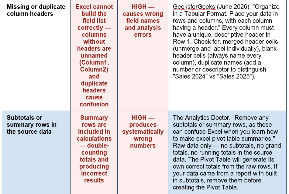
The quality of your Pivot Table depends entirely on the quality of your source data. The Analytics Doctor (December 2025): 'Preparing your data is the essential first step. Clean, well-structured data ensures your Pivot Tables work smoothly and return correct results.' Most Pivot Table failures — wrong totals, missing categories, COUNT instead of SUM — stem from data preparation errors, not from the Pivot Table itself. Before inserting a Pivot Table, verify all five of the following:

• Every column has a unique header in Row 1: The Pivot Table field list is built from your column headers. Missing headers produce unnamed columns (Column1, Column2). Duplicate headers cause confusion. GeeksforGeeks (June 2026): 'Organize in a Tabular Format: Place your data in rows and columns, with each column having a header.' Every column must be uniquely and descriptively named in Row 1.
• No blank rows or columns within the data: Excel uses blank rows and columns as boundaries — it treats everything before the first blank as the dataset. A blank row in the middle of your data will cause Excel to stop at that row, silently excluding everything below. GeeksforGeeks: 'Avoid Blank Rows or Columns: Ensure there are no empty rows or columns within your dataset.'
• No subtotals or grand total rows in the data: The Analytics Doctor: 'Remove any subtotals or summary rows, as these can confuse Excel.' If your data came from a report that includes subtotal rows (e.g. a monthly subtotal after each group of daily entries), delete them before creating the Pivot Table. The Pivot Table will generate its own correct totals.
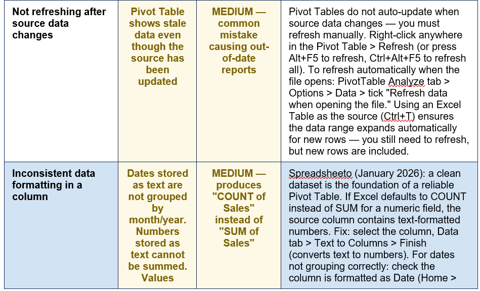
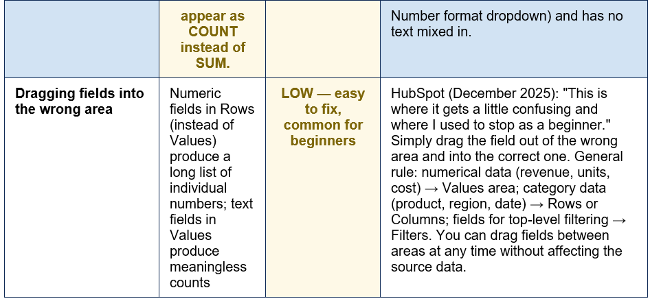
• Consistent data types within each column: All values in a date column should be dates (not a mix of dates and text). All values in a numeric column should be numbers (not a mix of numbers and text like 'N/A'). Mixed types cause Excel to default to COUNT aggregation instead of SUM for what should be a numeric field.
• Format as an Excel Table for best results: The Analytics Doctor: 'Select your data, then go to the Insert tab and choose Table. This step is crucial for anyone exploring how to make Pivot Table reports from dynamic data. Excel Tables automatically expand when you add new entries.' Formatting your source data as an Excel Table (Ctrl+T or Insert > Table) means that when you add new rows to the source data, they are automatically included in the Pivot Table on the next refresh — without manually extending the data range.

How to Create a Pivot Table: The Complete 7-Step Process

STEP 1 Click Anywhere in Your Dataset

Click any single cell within your data. Excel will automatically detect the extent of your data in the next step — you do not need to manually select all rows and columns before inserting the Pivot Table. TrumpExcel: 'Click anywhere in the dataset.' If your data is formatted as an Excel Table (Ctrl+T), Excel detects the table boundaries automatically. If not formatted as a Table, Excel uses the surrounding blank cells to detect the data range — which is why blank rows within your data cause problems.

STEP 2 Open the Create PivotTable Dialog

Go to the Insert tab on the Excel ribbon > click PivotTable (in the Tables group). Keyboard shortcut (Windows): Alt + N + V. Mac shortcut: Command + Option + P. GeeksforGeeks (June 2026): 'Select your Data >> Go to Insert Tab >> Select Pivot Table.' The 'Create PivotTable' dialog box opens. Spreadsheeto (January 2026): 'Go to the Insert Tab > Pivot Table to launch the Insert Pivot Table dialog box.'

STEP 3 Verify the Data Range and Choose a Location

In the dialog box: (a) Check the 'Table/Range' field shows the correct data range. TrumpExcel: 'It is filled in by default based on your data set. If your data has no blank rows or columns, Excel would automatically identify the correct range.' If it looks wrong, manually correct it. (b) Choose where to place the Pivot Table: 'New Worksheet' (recommended for beginners — places the Pivot Table on a clean sheet away from your data) or 'Existing Worksheet' (specify a cell location if you want the Pivot Table on the same sheet). Spreadsheeto: 'Check the option for a New Worksheet.' Click OK.

STEP 4 Understand the Empty Pivot Table and Field List Pane

After clicking OK, Excel creates a new worksheet with an empty Pivot Table placeholder on the left and the PivotTable Field List pane on the right. HubSpot (December 2025): 'You now have the skeleton of your Pivot Table, and it is time to flesh it out. This is where it gets a little confusing and where I used to stop as a beginner because I was so thrown off.' The Field List shows all your column headers as available fields at the top, and four areas at the bottom: Filters, Columns, Rows, and Values. Nothing appears in the Pivot Table yet — you need to drag fields into the areas.

STEP 5 Drag Fields into the Four Areas

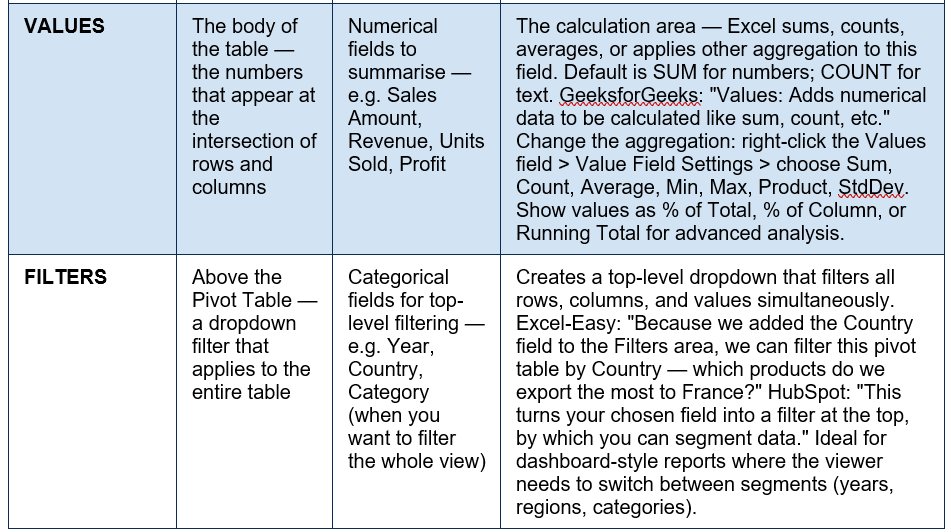
This is the core action: drag field names from the top of the Field List into the four areas. GeeksforGeeks: 'Rows: Sets rows for the table. Columns: Creates columns for our data. Values: Adds numerical data to be calculated. Filters: Adds filters to refine analysis.' Practical example using sales data: drag 'Product Name' to Rows (creates one row per product), drag 'Sales Amount' to Values (calculates sum of sales per product), drag 'Quarter' to Columns (shows sales by quarter across columns), drag 'Region' to Filters (adds a top-level region dropdown). You can drag fields in and out of areas at any time — the Pivot Table updates instantly without affecting the source data.

STEP 6 Customise the Calculation in the Values Area

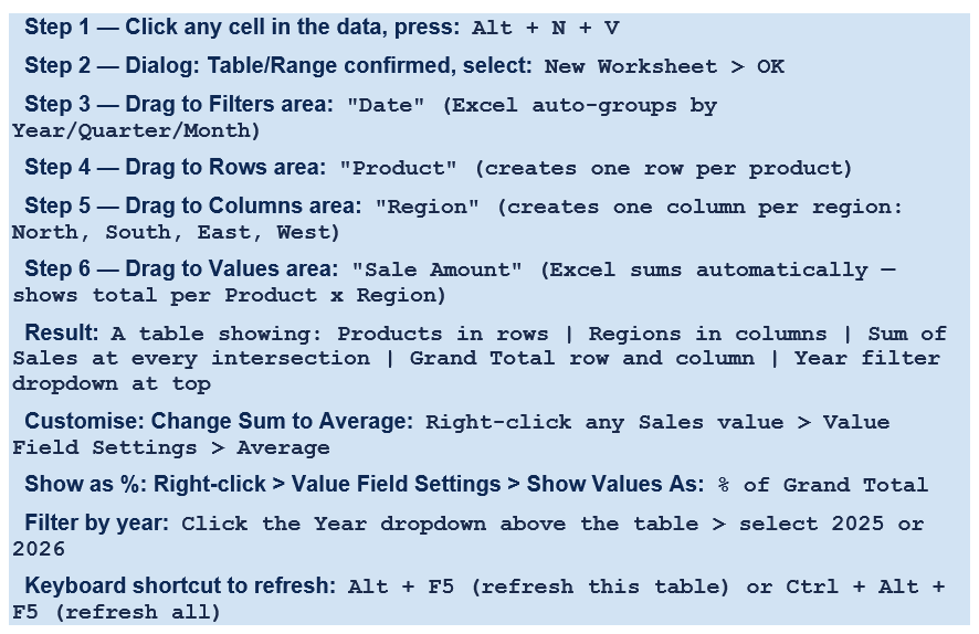
Excel defaults to SUM for numeric fields and COUNT for text fields. To change the calculation: right-click any value in the Values area of the Pivot Table > 'Value Field Settings.' GeeksforGeeks: 'Right-click on a value in the Values area and choose Value Field Settings. Then select the desired calculation.' Options: Sum, Count, Average, Min, Max, Product, Standard Deviation. To show values as percentages: in Value Field Settings > 'Show Values As' tab > choose '% of Grand Total', '% of Column Total', 'Running Total', or other comparative options. This is how the same Pivot Table shows both absolute and percentage views simultaneously.

STEP 7 Format, Sort, and Refresh

Format: Click the Pivot Table > PivotTable Analyze tab and Design tab appear in the ribbon. Under Design, choose a PivotTable Style for professional formatting. Number format the Values field: right-click the field > Value Field Settings > Number Format > choose Currency, Number with comma separator, or Percentage. Sort: Click the dropdown arrow next to any Row or Column label to sort A-Z, Z-A, or by value (largest to smallest, smallest to largest). Refresh: whenever source data changes, right-click the Pivot Table > Refresh (or press Alt+F5). Spreadsheeto: 'Whenever you make any changes to the source data, just refresh the Pivot Table and it will be reflected.' New rows are included automatically if source is an Excel Table.

The Four Pivot Table Areas: Complete Reference

Understanding the function of each area is the key to building any Pivot Table quickly. The following table maps all four areas with practical guidance on what to place in each: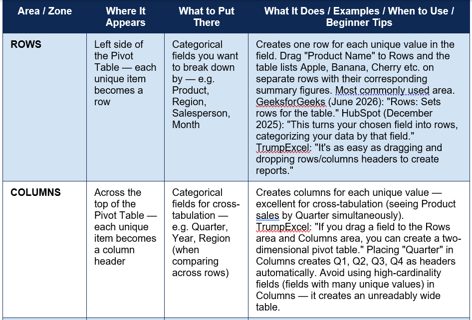

Complete Worked Example: Sales Data Pivot Table

The following example walks through building a complete, useful Pivot Table from scratch using a realistic sales dataset:




The Recommended PivotTables shortcut — let Excel suggest the layout: If you are unsure how to arrange your fields, use Excel's Recommended PivotTables feature. XelPlus (July 2026): 'If you are unsure how to start or want a quick way to explore your data, Excel's Recommended PivotTables feature is a great tool. Select your data, go to the Insert tab, click Tables, then Recommended PivotTables.' Excel analyses your data and suggests several ready-made layouts — click Preview to see how each looks, then click OK on the one that best answers your question. You can then modify the suggested layout by dragging fields in the Field List. This is the fastest way to get a useful starting point when you are new to Pivot Tables or when working with an unfamiliar dataset.

Excel Copilot and Pivot Tables in 2026: The New Way to Build

The most significant development in Pivot Table creation in 2026 is the integration of Microsoft 365 Copilot directly into Excel's Pivot Table workflow. XelPlus (2 weeks ago, July 2026): 'Microsoft 365 Copilot can build a Pivot Table from a plain English prompt. As of April 2026, Copilot's agentic mode is the default experience in Excel, meaning it edits your workbook directly instead of just suggesting steps.'

The prerequisites for using Copilot to build a Pivot Table: a Microsoft 365 Copilot subscription (Microsoft 365 Premium, Personal, or Family); data formatted as an Excel Table rather than a plain cell range; the file saved in OneDrive or SharePoint with AutoSave enabled. Once those conditions are met: click the Copilot icon on the Home tab and type a plain English request such as: Create a Pivot Table showing total sales by product and region. XelPlus: Copilot returns a draft with fields placed in Rows, Columns, Values, and Filters automatically. You can follow up with: Sort by sales largest to smallest, or Show values as percentage of grand total. Copilot adjusts the Pivot Table in place.

When to use Copilot versus building manually: XelPlus: 'Copilot is fastest for first drafts and exploratory analysis. Build manually when you need calculated fields, Power Pivot connections, or precise field placement.' For most everyday Pivot Table tasks — summarising sales, grouping by category, comparing periods — Copilot's natural language approach in 2026 eliminates the need to know which field goes in which area. For advanced analysis with calculated fields, custom groupings, or external data connections, manual construction gives more control.

The 6 Most Common Pivot Table Mistakes (And How to Fix Them)

Understanding what goes wrong — and why — is as important as knowing the steps. The following table maps the six errors that most commonly produce incorrect or incomplete Pivot Table results, with the specific fix for each: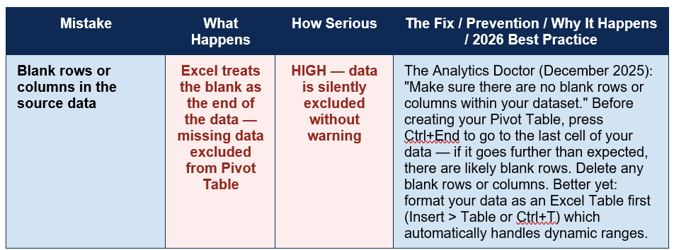

Beyond the Basics: Pivot Table Features That Transform Your Analysis

Once you have the basic Pivot Table working, several additional features significantly expand what you can do:

• Grouping dates by month, quarter, or year: When you drag a date field to Rows, right-click any date in the Pivot Table > Group > select Years, Quarters, Months (or multiple simultaneously). This creates automatic date hierarchy groupings without any formula. GeeksforGeeks (June 2026): multiple groupings can be applied to the same field simultaneously — click Year to expand to Quarter, Quarter to expand to Month.
• Calculated fields — create new metrics: PivotTable Analyze tab > Fields, Items & Sets > Calculated Field. Enter a formula using your existing fields. Example: if you have 'Revenue' and 'Cost' fields, create a Calculated Field for Profit = Revenue - Cost. This calculated field appears in the Values area like any other field but is computed dynamically across all categories.
• Slicers — visual interactive filters: PivotTable Analyze tab > Insert Slicer. Creates a visual button panel for filtering — much more user-friendly than the standard Filter dropdown. Multiple slicers can control multiple Pivot Tables simultaneously on a dashboard. Click a slicer button to filter; Ctrl+click for multiple selections; clear filter icon to reset.
• Timeline slicer for dates: PivotTable Analyze tab > Insert Timeline. Creates a visual date range selector — drag the handles to select a date period (month, quarter, year). Especially useful for financial reporting and sales dashboards where the user needs to switch between periods quickly.
• Show data as percentage of total: Right-click any value in the Values area > Show Values As > choose % of Grand Total, % of Column Total, or % of Row Total. This transforms absolute numbers into percentages without changing the underlying calculation — both views can exist in the same Pivot Table by adding the same field to Values twice with different Show Values As settings.
• Pivot Charts — visual representation: Select any cell in the Pivot Table > PivotTable Analyze tab > PivotChart. Creates a chart linked to the Pivot Table that updates when filters change. The chart type can be changed to bar, column, line, pie, or others. Particularly useful for presentations and dashboards where visualising the summary data is as important as the numbers themselves.

PIVOT TABLE KEYBOARD SHORTCUTS — THE ESSENTIAL CHEAT SHEET: Insert PivotTable dialog: Alt + N + V (Windows) | Command + Option + P (Mac). Refresh this Pivot Table: Alt + F5. Refresh all Pivot Tables in workbook: Ctrl + Alt + F5. Format as Table (before creating Pivot Table): Ctrl + T. Move between areas in Field List: Tab. Expand/collapse grouped fields: Alt + A + J (expand all) or Alt + A + H (collapse all). Open Field Settings dialog: from PivotTable, press Alt + JT + F. Select entire Pivot Table: Ctrl + A (click a cell in the Pivot Table first). Toggle Field List pane: PivotTable Analyze tab > Field List button. Add calculated field: PivotTable Analyze tab > Fields Items & Sets > Calculated Field.

Conclusion

A Pivot Table is the single most powerful data analysis tool available to most Excel users — and it requires no formulas, no programming, and no advanced Excel knowledge to produce genuinely useful results. The seven steps in this guide take any well-structured dataset from raw rows to a formatted, filterable summary in minutes: click in the data, press Alt+N+V, verify the range, choose New Worksheet, drag fields to the four areas, customise the Values calculation, and refresh when the data changes.

The foundations that make Pivot Tables work correctly — clean column headers, no blank rows, no subtotal rows, consistent data types, and data formatted as an Excel Table — are more important than any advanced feature. Most Pivot Table errors are data preparation errors, not tool errors. Get the data right before inserting the Pivot Table, and the tool does everything else.

In 2026, with Excel Copilot's agentic mode allowing plain English Pivot Table creation from a text prompt, the barrier to entry has dropped even further. For Microsoft 365 subscribers with their data in OneDrive, building a first-draft Pivot Table is now a single sentence. But understanding the four areas — Rows, Columns, Values, and Filters — and knowing how to customise, refresh, and extend a Pivot Table remains the skill that separates someone who can use a Pivot Table from someone who can use it well. This guide has given you both.

Frequently Asked Questions (FAQ)

What is a Pivot Table in Excel?

A Pivot Table is an interactive data summarisation tool built into Excel that lets you group, aggregate, and reorganise large datasets using a drag-and-drop interface — without formulas. XelPlus (July 2026): 'A Pivot Table in Excel is an easy way to summarise large amounts of data. It helps you find patterns and trends by organising data in a clear and simple layout. With a Pivot Table, you can arrange data in rows or columns and switch between these views easily. Excel calculates and shows summaries like totals, averages, or counts automatically.' Think of it as a dynamic reporting tool: you have 5,000 rows of sales transactions, and you want to see total sales by product, by region, or by month. Instead of writing SUMIF formulas or manually grouping rows, you drag the fields to the appropriate areas of the Pivot Table and Excel generates the summary instantly. The underlying data is never modified — the Pivot Table is only a view of it. You can change the layout at any time by dragging fields to different areas, and the Pivot Table updates in real time.

How do I insert a Pivot Table in Excel?

Inserting a Pivot Table in Excel takes four steps. (1) Click any cell within your data. (2) Go to the Insert tab in the Excel ribbon and click PivotTable (in the Tables group). Keyboard shortcut on Windows: Alt + N + V. Keyboard shortcut on Mac: Command + Option + P (GeeksforGeeks, June 2026). (3) In the Create PivotTable dialog that appears: verify the Table/Range shows the correct data range; select 'New Worksheet' (recommended for beginners); click OK. (4) The new worksheet opens with an empty Pivot Table and the Field List pane on the right. Drag fields from the top of the Field List into the Rows, Columns, Values, and Filters areas to build your summary. Spreadsheeto (January 2026): 'Go to the Insert Tab > Pivot Table (Or press the Alt Key > N > V) to launch the Insert Pivot Table dialog box.' The entire process from click to first meaningful summary takes approximately 2-3 minutes once you understand the four areas.

Why does my Pivot Table show COUNT instead of SUM?

When a Pivot Table shows COUNT of a field instead of SUM, it means Excel detected text values (not pure numbers) in the column you dragged to the Values area. This happens because: some cells in the column contain text (the word 'N/A', blank cells treated as text, or numbers formatted as text rather than actual numeric values). Excel defaults to SUM for numeric columns and COUNT for any column that contains text — even one text cell in an otherwise numeric column causes the entire field to be counted rather than summed. To fix it: (1) Go back to your source data. Select the entire column. Check for any non-numeric entries — blanks, text like 'N/A', dashes. Replace or delete them. (2) If numbers are formatted as text: select the column, go to Data tab > Text to Columns > click Finish immediately (this converts text-formatted numbers back to true numbers). (3) After fixing the source data, refresh the Pivot Table (right-click > Refresh). The field should now sum correctly. Alternatively, change the calculation inside the Pivot Table: right-click any value in the Values area > Value Field Settings > Sum (if the option is available after fixing the data).

How do I refresh a Pivot Table when data changes?

Pivot Tables do not automatically update when the source data changes — you must refresh them manually. The three ways to refresh: (1) Right-click anywhere inside the Pivot Table > Refresh. (2) Keyboard shortcut: Alt + F5 (refreshes the current Pivot Table); Ctrl + Alt + F5 (refreshes all Pivot Tables in the workbook). (3) PivotTable Analyze tab > Refresh button (dropdown offers Refresh or Refresh All). To set the Pivot Table to refresh automatically when the file is opened: go to PivotTable Analyze tab > Options > Data > tick 'Refresh data when opening the file.' Spreadsheeto (January 2026): 'Whenever you make any changes to the source data, just refresh the Pivot Table and it will be reflected.' Important note: if you have added new rows to the source data, they will only be included after refreshing IF the source data is formatted as an Excel Table (Ctrl+T). Plain cell ranges do not automatically expand when new rows are added — the Pivot Table only sees the original range unless you update the data source manually (PivotTable Analyze > Change Data Source).

Can Excel Copilot create a Pivot Table for me in 2026?

Yes — as of April 2026, Microsoft 365 Copilot can build a Pivot Table from a plain English prompt in its agentic mode, which edits the workbook directly. XelPlus (2 weeks ago, July 2026): 'Microsoft 365 Copilot can build a Pivot Table from a plain English prompt. As of April 2026, Copilot's agentic mode is the default experience in Excel, meaning it edits your workbook directly instead of just suggesting steps.' Requirements to use Copilot for Pivot Tables: a Microsoft 365 Copilot subscription (Microsoft 365 Premium, Personal, or Family); your data formatted as an Excel Table (Insert > Table or Ctrl+T); the file saved in OneDrive or SharePoint with AutoSave on. Process: click the Copilot icon on the Home tab, type your request (e.g. 'Create a Pivot Table showing total revenue by product and region'), and Copilot places the fields in Rows, Columns, Values, and Filters automatically. You can then follow up with natural language adjustments: 'Sort by revenue largest to smallest' or 'Show values as percentage of grand total.' XelPlus: 'Copilot is fastest for first drafts and exploratory analysis. Build manually when you need calculated fields, Power Pivot connections, or precise field placement.' Without a Copilot subscription, Excel still offers the Recommended PivotTables feature (Insert > Recommended PivotTables) which suggests ready-made layouts based on your data structure.