Table of Contents

• The 30 Most-Used Excel Formulas: Quick Reference Table
• Category 1: Mathematics and Statistical Formulas (1–30)
• Core Arithmetic and Aggregation
• Rounding and Number Formatting
• Counting Functions
• Category 2: Logical Functions (31–50)
• IF and Its Variants
• Category 3: Lookup and Reference Formulas (51–80)
• VLOOKUP, HLOOKUP and Their Limitations
• Reference and Navigation Functions
• Modern Dynamic Array Lookups
• Category 4: Text and String Formulas (81–110)
• Cleaning and Standardising Text
• Extracting and Splitting Text
• Category 5: Date and Time Formulas (101–120)
• Category 6: Financial Formulas (121–140)
• Category 7: Advanced and Dynamic Array Formulas (141–150)
• Practical Tips for Excel Formula Mastery
• Conclusion
• Frequently Asked Questions (FAQ)
• External References & Further Reading

Excel is the world's most widely used spreadsheet application, and the gap between someone who knows a handful of formulas and someone who has genuinely mastered its function library is one of the most economically valuable skills gaps in professional life. A LinkedIn Workforce Report found that Excel skills appear in job postings more than almost any other software tool, and surveys consistently show that proficiency in Excel formulas is among the top three skills employers request in roles spanning finance, operations, marketing, HR, project management, and data analysis.

The challenge for most learners is that Excel has over 500 built-in functions — a number that has grown substantially in recent years with the introduction of dynamic array functions like FILTER, UNIQUE, SORT, and SEQUENCE in Excel 365. No single guide can cover all 500 in depth. What this guide does instead is provide a structured, example-driven walkthrough of the 150 formulas and function families that real-world Excel users reach for most frequently, organised by category, with syntax, a worked example, and a practical note for each one.

Whether you are starting from scratch with SUM and IF, working toward confident use of VLOOKUP and INDEX/MATCH, or ready to explore the modern dynamic array functions that have transformed what Excel can do in a single formula, this guide provides the structured reference you need. The 30 most-used formulas are presented in a quick-reference table; the remaining categories are covered in depth section by section, with real-world scenarios for each formula family.

The 30 Most-Used Excel Formulas: Quick Reference Table

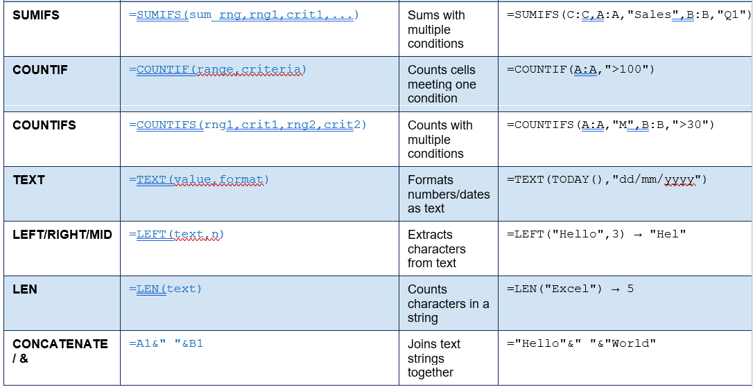
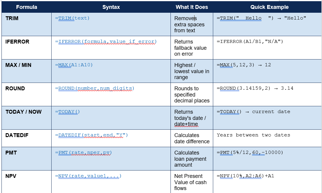
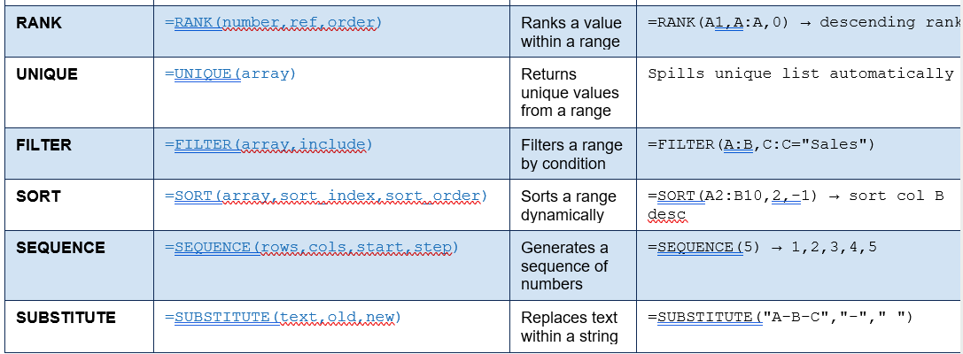
The table below covers the 30 formulas that appear in the widest range of real-world Excel files, from beginner spreadsheets to complex financial models. Each entry shows the syntax, what it does, and a quick example: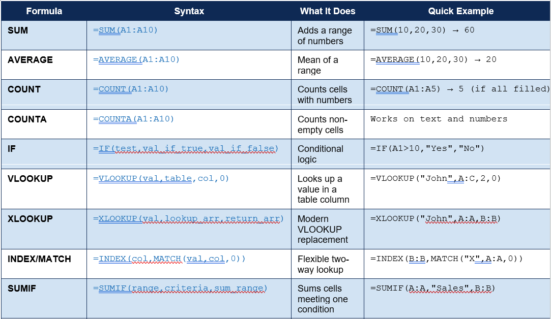






The most searched Excel formula globally: VLOOKUP — over 5 million monthly searches — despite being largely superseded in Excel 365 by XLOOKUP, VLOOKUP remains the most searched Excel function worldwide as of 2026, reflecting both the enormous installed base of older Excel versions and the continued dominance of lookup formulas in everyday spreadsheet work

Category 1: Mathematics and Statistical Formulas (1–30)

Mathematical and statistical functions form the foundation of almost every Excel spreadsheet. Beyond the basic SUM and AVERAGE that most users know, this category includes powerful aggregation tools that can transform how you analyse data.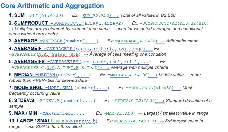

Counting Functions

21. COUNT =COUNT(value1,...) Ex: =COUNT(A1:A20) → Counts cells containing numbers only

22. COUNTA =COUNTA(value1,...) Ex: =COUNTA(A1:A20) → Counts all non-empty cells including text

23. COUNTBLANK =COUNTBLANK(range) Ex: =COUNTBLANK(A1:A20) → Counts empty cells — useful for data quality checks

24. COUNTIF =COUNTIF(range,criteria) Ex: =COUNTIF(A:A,"100") → Count of cells exceeding 100

25. COUNTIFS =COUNTIFS(rng1,crit1,rng2,crit2,...) Ex: =COUNTIFS(A:A,"Sales",B:B,"2026") → Multi-condition count

26. FREQUENCY =FREQUENCY(data_array,bins_array) Ex: =FREQUENCY(A1:A100,{10,20,30}) → Array formula returning frequency distribution in bins

27. RANK.EQ =RANK.EQ(number,ref,order) Ex: =RANK.EQ(A1,A:A,0) → Rank of a value — order 0 = descending (highest = rank 1)

28. PERCENTILE.INC =PERCENTILE.INC(array,k) Ex: =PERCENTILE.INC(A1:A100,0.9) → 90th percentile of the dataset

29. QUARTILE.INC =QUARTILE.INC(array,quart) Ex: =QUARTILE.INC(A1:A100,1) → 1st quartile (25th percentile)

30. SUMPRODUCT with conditions =SUMPRODUCT(--(A:A="UK"),B:B) Ex: =SUMPRODUCT(--(A2:A100="UK"),B2:B100) → Conditional sum without SUMIFS — the -- converts TRUE/FALSE to 1/0

Why SUMPRODUCT is a power user's favourite: SUMPRODUCT can replicate SUMIFS, COUNTIFS, and even complex multi-condition aggregations in a single formula without needing Ctrl+Shift+Enter. The pattern =SUMPRODUCT(--(condition1),--(condition2),values) is one of the most versatile patterns in Excel, particularly valuable when working with older versions that lack some modern functions.

Category 2: Logical Functions (31–50)

Logical functions let you make decisions in your spreadsheet. They are the 'if this, then that' engine of Excel and underpin most sophisticated data analysis models.

IF and Its Variants

31. IF =IF(logical_test,value_if_true,value_if_false) Ex: =IF(A11000,"High","Low") → Returns 'High' if A1 exceeds 1,000
32. IFS =IFS(test1,val1,test2,val2,...) Ex: =IFS(A190,"A",A180,"B",A170,"C",TRUE,"F") → Multiple conditions without nesting — available Excel 2019+
33. NESTED IF =IF(A190,"A",IF(A180,"B",IF(A170,"C","F"))) Ex: =IF(A190,...) → Classic nested approach — use IFS where available as it is more readable
34. IFERROR =IFERROR(value,value_if_error) Ex: =IFERROR(VLOOKUP(A1,B:C,2,0),"Not Found") → Returns 'Not Found' if lookup fails — prevents #N/A and #DIV/0! errors
35. IFNA =IFNA(value,value_if_na) Ex: =IFNA(XLOOKUP(A1,B:B,C:C),"Missing") → Catches #N/A errors only — more precise than IFERROR
36. AND =AND(logical1,logical2,...) Ex: =AND(A10,B10,C1100) → TRUE only if ALL conditions are true
37. OR =OR(logical1,logical2,...) Ex: =OR(A1="Sales",A1="Marketing") → TRUE if ANY condition is true
38. NOT =NOT(logical) Ex: =NOT(ISBLANK(A1)) → TRUE if A1 is NOT blank
39. XOR =XOR(logical1,logical2,...) Ex: =XOR(A150,B150) → TRUE if an ODD number of conditions are true
40. SWITCH =SWITCH(expression,val1,result1,...) Ex: =SWITCH(A1,1,"Jan",2,"Feb",3,"Mar") → Matches an expression against multiple values — cleaner than nested IFs for fixed lists
41. IF with AND =IF(AND(A10,B10),"Both Positive","Check values") Ex: =IF(AND(A10,B10),...) → Combining logical functions — works for any number of combined conditions
42. ISBLANK =ISBLANK(value) Ex: =ISBLANK(A1) → TRUE if cell is truly empty
43. ISNUMBER =ISNUMBER(value) Ex: =ISNUMBER(A1) → TRUE if cell contains a number — useful after text imports
44. ISTEXT =ISTEXT(value) Ex: =ISTEXT(A1) → TRUE if cell contains text
45. ISERROR =ISERROR(value) Ex: =ISERROR(A1/B1) → TRUE if value returns any error type
46. ISNA =ISNA(value) Ex: =ISNA(VLOOKUP(A1,B:C,2,0)) → TRUE if value returns #N/A specifically
47. LET =LET(name,val,calculation) Ex: =LET(x,A1*B1,x+x*0.2) → Assigns names to values within a formula — reduces repetition and improves readability
48. LAMBDA =LAMBDA(param,formula) Ex: =LAMBDA(x,x^2+2*x+1) → Creates reusable custom functions without VBA — Excel 365 / 2021+
49. BYCOL / BYROW =BYCOL(array,LAMBDA(col,SUM(col))) Ex: =BYCOL(A1:D5,...) → Applies a LAMBDA to each column or row — powerful for dynamic summaries
50. TRUE() / FALSE() =IF(A1=TRUE(),"Yes","No") Ex: =TRUE() → Returns the logical values TRUE or FALSE — rarely needed directly but useful in formula construction

Category 3: Lookup and Reference Formulas (51–80)

Lookup functions are the most frequently cited source of Excel frustration — and the most transformative once mastered. They allow you to retrieve data from one part of a workbook based on a value in another, which is the foundation of virtually every data-matching and reporting task.

VLOOKUP, HLOOKUP and Their Limitations

51. VLOOKUP (exact match) =VLOOKUP(lookup_value,table_array,col_index,0) Ex: =VLOOKUP("Smith",A:D,3,0) → Returns value from column 3 of A:D where column A = 'Smith'. The 0 (or FALSE) specifies exact match.
52. VLOOKUP (approximate match) =VLOOKUP(lookup_value,table_array,col_index,1) Ex: =VLOOKUP(85,A:B,2,1) → Finds the largest value = 85 in column A — used for tax bands, commission tiers, and grade lookups. Table must be sorted ascending.
53. HLOOKUP =HLOOKUP(lookup_value,table_array,row_index,0) Ex: =HLOOKUP("Q1",A1:D5,3,0) → Like VLOOKUP but searches horizontally across rows
54. XLOOKUP (basic) =XLOOKUP(lookup_value,lookup_array,return_array) Ex: =XLOOKUP("Smith",A:A,C:C) → Modern replacement for VLOOKUP — no column number needed, works left and right
55. XLOOKUP with not-found =XLOOKUP(val,lookup_arr,return_arr,"Not Found") Ex: =XLOOKUP(A1,B:B,C:C,"N/A") → Built-in error handling — fourth argument replaces IFERROR wrapper
56. XLOOKUP (last match) =XLOOKUP(val,lookup_arr,return_arr,,-1) Ex: =XLOOKUP(A1,B:B,C:C,,-1) → Searches from last to first — finds most recent match
57. XLOOKUP (wildcard) =XLOOKUP("*"&A1&"*",B:B,C:C,,2) Ex: =XLOOKUP("*Smith*",A:A,B:B,,2) → Partial text match — match mode 2 enables wildcards
58. INDEX =INDEX(array,row_num,col_num) Ex: =INDEX(B2:D20,3,2) → Returns value at row 3, column 2 of the range B2:D20
59. MATCH =MATCH(lookup_value,lookup_array,match_type) Ex: =MATCH("Smith",A:A,0) → Returns position of 'Smith' in column A — combine with INDEX for flexible lookup
60. INDEX/MATCH (combined) =INDEX(return_col,MATCH(val,lookup_col,0)) Ex: =INDEX(C:C,MATCH(A1,A:A,0)) → The traditional power-user alternative to VLOOKUP — works left, right, and on unsorted data
61. INDEX/MATCH/MATCH (2D) =INDEX(table,MATCH(row_val,row_col,0),MATCH(col_val,header_row,0)) Ex: =INDEX(B2:D10,MATCH(A15,A2:A10,0),MATCH(B15,B1:D1,0)) → Two-way lookup — finds the intersection of a matching row AND column

Reference and Navigation Functions

62. OFFSET =OFFSET(reference,rows,cols,height,width) Ex: =OFFSET(A1,2,1) → Returns a range offset from a starting point — powerful for dynamic named ranges
63. INDIRECT =INDIRECT(ref_text) Ex: =INDIRECT("Sheet2!A1") → Converts text to a cell reference — useful for dynamic sheet references
64. ADDRESS =ADDRESS(row_num,col_num) Ex: =ADDRESS(3,2) → Returns '$B$3' — the address of row 3, column 2
65. ROW / ROWS =ROW(reference) Ex: =ROW(A5) → 5 — returns the row number. ROWS counts total rows in a range.
66. COLUMN / COLUMNS =COLUMN(reference) Ex: =COLUMN(C1) → 3 — returns the column number
67. CHOOSE =CHOOSE(index_num,val1,val2,...) Ex: =CHOOSE(2,"Jan","Feb","Mar") → 'Feb' — returns the nth item from a list based on the index number
68. HYPERLINK =HYPERLINK(link_location,friendly_name) Ex: =HYPERLINK("https://example.com","Click here") → Creates a clickable hyperlink in a cell
69. GETPIVOTDATA =GETPIVOTDATA(data_field,pivot_table,...) Ex: Auto-generated when clicking pivot table cells → Retrieves specific data from a PivotTable — useful for dynamic reports
70. FORMULATEXT =FORMULATEXT(reference) Ex: =FORMULATEXT(B1) → Shows the formula in B1 as text — excellent for formula auditing and documentation

Modern Dynamic Array Lookups

71. FILTER =FILTER(array,include,if_empty) Ex: =FILTER(A2:C100,B2:B100="Sales","No results") → Returns all rows where column B equals 'Sales' — spills results automatically
72. UNIQUE =UNIQUE(array,by_col,exactly_once) Ex: =UNIQUE(A2:A100) → Returns distinct values from a range — foundation for dynamic dropdown lists
73. SORT =SORT(array,sort_index,sort_order,by_col) Ex: =SORT(A2:C50,3,-1) → Sorts by column 3 descending — dynamic, updates automatically as data changes
74. SORTBY =SORTBY(array,by_array1,sort_order1,...) Ex: =SORTBY(A2:B50,B2:B50,-1) → Sorts by an external column not necessarily in the return range
75. XMATCH =XMATCH(lookup_value,lookup_array,match_mode) Ex: =XMATCH("Smith",A:A,0) → Modern MATCH replacement — supports wildcards and binary search; returns position
76. TAKE / DROP =TAKE(array,rows,cols) Ex: =TAKE(A1:D100,5) → Returns the first 5 rows of the range — DROP removes rows from start or end
77. CHOOSEROWS / CHOOSECOLS =CHOOSEROWS(array,row1,row2,...) Ex: =CHOOSEROWS(A1:D10,1,3,5) → Returns specific rows — use for extracting non-contiguous rows
78. VSTACK / HSTACK =VSTACK(array1,array2) Ex: =VSTACK(A1:B5,D1:E5) → Stacks two ranges vertically into one — no longer need copy-paste to combine datasets
79. TOCOL / TOROW =TOCOL(array,ignore) Ex: =TOCOL(A1:D5) → Converts a 2D range into a single column — ignore 1 skips blanks
80. MAKEARRAY =MAKEARRAY(rows,cols,LAMBDA(r,c,formula)) Ex: =MAKEARRAY(5,3,LAMBDA(r,c,r*c)) → Generates an array of any size using a formula — very powerful for modelling

The VLOOKUP vs XLOOKUP decision: If you are using Excel 2021 or Microsoft 365, default to XLOOKUP for new lookups. It searches both left and right, does not require column numbers, has built-in error handling, and is faster on large datasets. If you need to share files with users on Excel 2016 or earlier, VLOOKUP remains the safer compatibility choice — or pair INDEX/MATCH which works in all modern versions.

Category 4: Text and String Formulas (81–110)

Text functions are essential for cleaning imported data, standardising formats, extracting specific information from cells, and building dynamic labels and descriptions. Most real-world Excel files involve at least some text manipulation.

Cleaning and Standardising Text

81. TRIM =TRIM(text) Ex: =TRIM(" Hello World ") → 'Hello World' — removes leading, trailing, and excess internal spaces
82. CLEAN =CLEAN(text) Ex: =CLEAN(A1) → Removes non-printable characters — essential for data imported from databases or PDFs
83. UPPER / LOWER / PROPER =PROPER(text) Ex: =PROPER("john smith") → 'John Smith' — title-case conversion; UPPER = ALL CAPS; LOWER = all lower
84. SUBSTITUTE =SUBSTITUTE(text,old_text,new_text,instance) Ex: =SUBSTITUTE(A1,"-","") → Removes all hyphens — use instance parameter to replace only the nth occurrence
85. REPLACE =REPLACE(old_text,start,num_chars,new_text) Ex: =REPLACE("AB123",1,2,"XX") → 'XX123' — replaces characters at a specific position
86. FIND / SEARCH =FIND(find_text,within_text,start_num) Ex: =FIND("@",A1) → Position of '@' in A1 — FIND is case-sensitive; SEARCH allows wildcards
87. VALUE =VALUE(text) Ex: =VALUE("1,234") → 1234 — converts a number stored as text into a true number
88. TEXT =TEXT(value,format_text) Ex: =TEXT(DATE(2026,7,4),"dd mmmm yyyy") → '04 July 2026' — formats any value as a text string
89. NUMBERVALUE =NUMBERVALUE(text,decimal_sep,group_sep) Ex: =NUMBERVALUE("1.234,56",",",".") → Converts European number formats to Excel numbers
90. REPT =REPT(text,number_times) Ex: =REPT("*",5) → '*****' — repeats a character n times; useful for in-cell bar charts

Extracting and Splitting Text

91. LEFT =LEFT(text,num_chars) Ex: =LEFT("Product-A12",7) → 'Product'
92. RIGHT =RIGHT(text,num_chars) Ex: =RIGHT("REF-2026",4) → '2026'
93. MID =MID(text,start_num,num_chars) Ex: =MID("ABCDEF",3,2) → 'CD' — starts at position 3, extracts 2 characters
94. LEN =LEN(text) Ex: